HC
The core problem: a forced trade-off
Residual connections (the output = layer(input) + input pattern) have been the workhorse of deep networks since ResNet. They solve one big problem — gradient vanishing — by giving gradients a clean highway back through the network during backprop.
But where you put the normalization inside that pattern creates a forced choice between two failure modes, and you can’t escape both:
Pre-Norm (output = layer(norm(input)) + input)
- Gradients flow well — training is stable, deep networks train fine
- Causes representation collapse: as you stack more layers, the hidden states in deep layers become nearly identical to each other. Each additional layer contributes less and less. You can see this directly in Figure 3 of the paper — for OLMo-1B with Pre-Norm, the cosine similarity between adjacent layers’ inputs is ~0.9+ in deeper layers. The layers are barely doing anything new.
Post-Norm (output = norm(layer(input) + input))
- Each layer’s contribution stays distinct — no collapse
- Gradients shrink as they pass back through each norm, so gradient vanishing returns. Deep networks become hard to train.
The paper calls this the seesaw effect: push down on one problem, the other one pops up. You can’t have both.
The deeper issue the paper identifies: residual connections hardcode the strength of the connection between a layer’s input and output. The weight is always 1. The network doesn’t get to decide.
Pre-Norm and Post-Norm are really just two different fixed recipes for this connection. Neither is learned. Neither adapts. The network is stuck with whatever trade-off the architect picked, the same trade-off at every layer, for every input.
That’s the limitation hyper-connections attacks head-on. The driving question in the paper: Can neural networks autonomously learn the optimal strength of connections to improve performance?
What hyper-connections actually fixes
Make connection strengths learnable. Instead of a fixed weight of 1, let the network learn how much of the input vs. the layer output should flow forward, per layer. The paper shows Pre-Norm and Post-Norm are just specific non-trainable instances of their more general matrix — so HC is a strict generalization, not a different thing.
Give the network multiple “lanes” (n > 1). A single learnable weight per layer isn’t enough — the seesaw still exists with one hidden state (and their n=1 experiments confirm this: DHC×1 actually performs worse than baseline). By keeping n parallel copies of the hidden state, the network can maintain different connection patterns simultaneously: one lane can carry long-range information Pre-Norm style, another can do short-range Post-Norm style. You get both behaviors at once instead of trading them off.
Let the arrangement adapt per token (DHC). Once connection weights are learnable, specific values correspond to specific layer arrangements — sequential, parallel, or mixtures. With dynamic weights, the network can effectively rearrange its own layers depending on what token it’s processing.
Pre-Norm: addresses gradient vanishing, but introduce representation collapse (similar representation, rank collapse). Post-Norm: alleviates the issue of representation collapse but still has gradient vanishing problem.
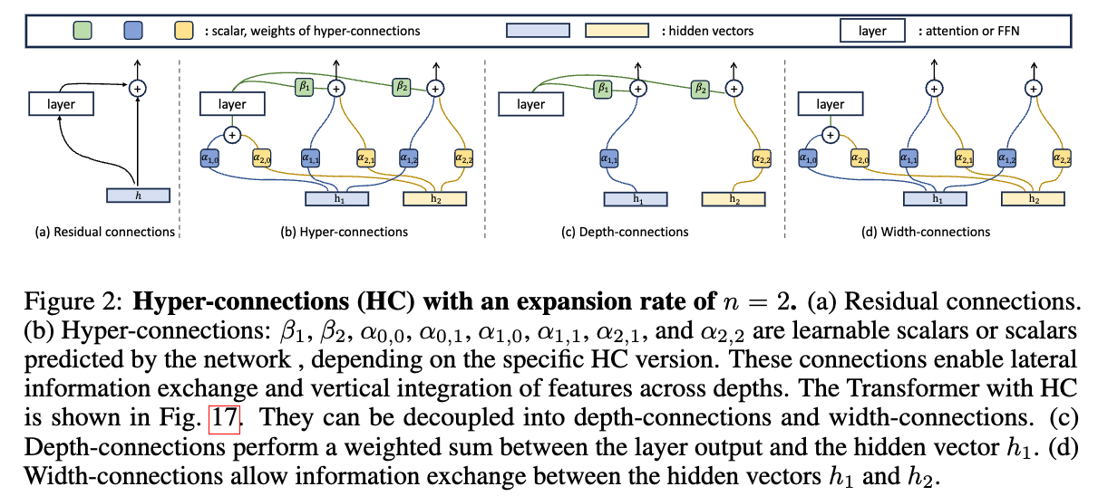
Residual Connections
In a standard transformer, every layer does the same thing:
output = layer(input) + input
The “+ input” is the residual connection. The weight is hardcoded to 1. The network has no say in how much of the input vs. the layer output should flow forward. Pre-Norm and Post-Norm just pick different fixed recipes for this, and each has a downside (gradient vanishing vs. representation collapse — the “seesaw” the paper keeps mentioning). In other words, residual connections are rigid
Static HC
Instead of one hidden vector flowing through the network, HC keeps n parallel copies of the hidden state (called the “hyper hidden matrix” H). At each layer, two things happen, both controlled by learnable scalar weights:
- Width connections (matrix
Am,Ar): mix the n hidden vectors with each other to produce the input to this layer, and to produce the n hidden vectors that get passed forward. - Depth connections (matrix
B): decide how much of the layer’s output gets added to each of the n hidden vectors.
So instead of one rigid “+ input”, you have an (n+1) × (n+1) matrix of learnable weights deciding how information flows. Pre-Norm and Post-Norm turn out to be special non-trainable cases of this matrix (Section 3.1 of the paper).
The key word here is learnable but fixed after training. SHC learns the weights during pre-training, then they’re frozen. Every token sees the same connection pattern.
Dynamic HC
DHC takes the next step: the connection weights depend on the input itself. Different tokens get different connection patterns.
Mechanically:
H_norm = norm(H)                           # normalize the hidden state
B(H)   = s_β  · tanh(H_norm · W_β) + B     # dynamic depth weights
Am(H)  = s_α  · tanh(H_norm · W_m) + Am    # dynamic width weights (input side)
Ar(H)  = s_α  · tanh(H_norm · W_r) + Ar    # dynamic width weights (residual side)
Reading that right-to-left for each line: you start with the static learned matrix (B, Am, Ar), and you add a small input-dependent correction. The correction is computed by:
- Normalizing the current hidden state
- Linearly projecting it to produce raw weights
- Squashing through
tanhto bound them - Scaling by a small learnable factor
s(initialized to 0.01, so it starts barely perturbing the static weights)
The W_β, W_m, W_r projection matrices are initialized to zero, so at the start of training DHC behaves exactly like SHC (which itself is initialized to behave like Pre-Norm). The dynamic behavior emerges as training progresses.
Dynamic layer rearrangement
This is the conceptual payoff. Section 3.2 shows that specific HC matrix values correspond to arranging layers sequentially vs. in parallel (like parallel attention+FFN blocks). Since DHC’s matrix changes per token, the network can effectively rearrange its own layers on the fly — running some layers in parallel for one token, sequentially for another, or in some soft mixture.
The visualization in Figure 7 and Appendix F backs this up: trained DHC models show a “Λ-shaped” connection pattern that’s a learned mixture of Pre-Norm and Post-Norm styles, with parallel-transformer-block patterns popping up spontaneously in certain layer ranges.
DHC vs SHC empirically
Table 2 of the paper: at expansion rate n=2, DHC and SHC perform similarly. At n=4, DHC pulls ahead noticeably. So the dynamic component is most useful when you have more hidden-state “lanes” for it to route between — which makes intuitive sense, since with more lanes there’s more meaningful routing to do.
DHC = static hyper-connections (a learnable mixing matrix replacing the fixed residual) plus a small input-dependent correction to that matrix, letting the network choose its connection pattern (and effectively its layer arrangement) per token, at near-zero extra cost.
Two concrete signals from the paper shows the idea works:
- Representation collapse goes away. Figure 3: with hyper-connections, the cosine similarity between adjacent layers drops dramatically and varies much more. Each layer is doing distinct work again.
- Training is more stable. The 7B baseline shows frequent loss spikes during training; the HC version shows none (Figure 6). And convergence is faster — OLMoE-1B-7B with DHC×4 hits the baseline’s 500B-token loss in roughly half the tokens.
For OLMo-1B-DHC×4, DHC adds about 0.03% more parameters and 0.2% more FLOPs (Tables 7 and 8). The dynamic projections (W_β, W_m, W_r) are the bulk of the added parameters but they’re small linear maps from d_model to n or n×n.
HC to mHC
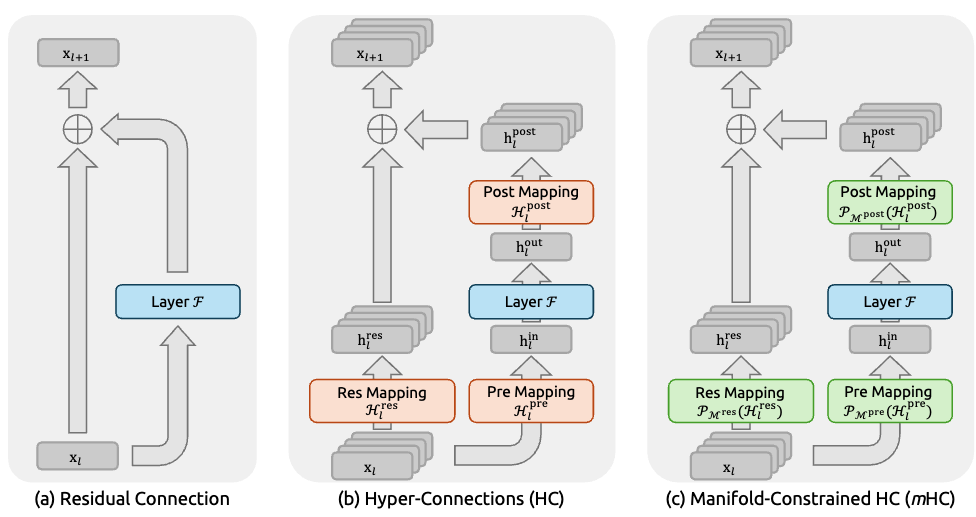
DeepSeek evolves hyper-connection to Manifold-Constrained Hyper-Connections.
What broke when HC scaled up
The original HC paper showed strong results up to 7B parameters trained on 500B tokens. Those are real numbers, but they’re not frontier scale. When DeepSeek tried to push HC further — to 27B MoE models trained at production scale — two problems surfaced that didn’t show up clearly at smaller scales:
- Problem 1: The identity mapping property is gone.
Recall how a plain residual connection composes across layers:
x_L = x_l + Σ F(x_i)
That x_l term sitting there unchanged across L−l layers is the identity mapping, and it’s what keeps gradients flowing cleanly back to early layers. ResNet’s authors identified this as the whole reason deep residual nets train at all.
HC composes differently:
x_L = (∏ H_res) · x_l + Σ (∏ H_res) · H_post · F(...)
That product of residual mapping matrices ∏ H_res is a learnable n×n matrix multiplied across every layer. It is not the identity. Since each H_res is unconstrained, the product can amplify or shrink the signal arbitrarily.
The empirical damage is striking (Figure 3 of the mHC paper): in a 27B HC model, the composite mapping’s signal gain hits ~3000× at some layers, when it should be near 1. That’s three orders of magnitude away from identity. Gradient norms become erratic, and loss spikes appear around step 12k. The seesaw that HC was meant to solve gets replaced by a different instability — exploding/vanishing signals through the composite mapping.
- Problem 2: Memory access and pipeline cost is real at scale.
The original HC paper argued FLOPs overhead is negligible, which is true. But the n-stream residual reads and writes n× more data per layer, and in pipeline parallelism it sends n× more across stages. FLOPs aren’t the bottleneck in modern LLM training; memory bandwidth and inter-stage communication are. The original paper didn’t address this because at 7B with conventional parallelism.
The mHC fix
The conceptual move is: keep HC’s expressivity, but constrain H_res so its composition stays well-behaved.
Specifically, they project H_res onto the Birkhoff polytope — the set of doubly stochastic matrices (non-negative entries, every row sums to 1, every column sums to 1). This is done with the Sinkhorn-Knopp algorithm (20 iterations of alternating row/column normalization on exp(H_res)).
Three properties fall out of this choice, and they’re the whole argument:
Norm preservation. The spectral norm of a doubly stochastic matrix is bounded by 1. So a single layer can never amplify the signal — gradient explosion through
H_resis structurally impossible.Compositional closure. Product of doubly stochastic matrices is doubly stochastic. So
∏ H_resalso has spectral norm ≤ 1. The stability holds no matter how deep the network goes.Geometric meaning. A doubly stochastic matrix is a convex combination of permutation matrices. So
H_res · xis literally a mixing operation — features get blended across the n streams in a way that conserves the global mean. This restores something morally equivalent to the identity mapping: the average signal energy across streams is conserved, even though individual streams still mix.
They also constrain H_pre and H_post to be non-negative (via sigmoid), to prevent sign cancellation across streams.
The result (Figure 7): single-layer gain stays near 1.0, composite gain peaks around 1.6 instead of 3000. Three orders of magnitude reduction in instability.
The 1×1 special case
This is the small detail that makes the framing click. When n=1, a doubly stochastic 1×1 matrix is just the scalar 1. So mHC at n=1 degenerates exactly to the original residual connection’s identity mapping. mHC is positioned as the principled generalization: HC widened the residual stream and broke identity; mHC restores identity while keeping the width.
The engineering half of the paper
Sections 4.3 and Figure 4 are mostly about making mHC affordable at scale. The headline number: with all the optimizations, mHC adds only 6.7% training overhead at n=4 on their 27B setup. The optimizations are:
- Kernel fusion via TileLang. They fuse the dynamic mapping computations, the Sinkhorn-Knopp iteration, and the residual merge into a small number of GPU kernels. Notably they derive a custom backward kernel for Sinkhorn that recomputes the iteration on-chip rather than storing 20 intermediate matrices.
- Selective recomputation. Don’t store the n-stream intermediates — recompute them in the backward pass from a single cached input every L_r layers. They derive an optimal block size L_r ≈ √(nL/(n+2)).
- DualPipe scheduling. Overlap the extra communication from the n-stream residual with computation by running mHC kernels on a dedicated high-priority CUDA stream.
This is the part of the paper that wouldn’t exist if HC had stayed at the 7B/500B-token scale of the original paper.
mHC Results
At 27B, against the baseline (plain residual): mHC beats it on all 8 benchmarks. Against HC: mHC matches or beats HC on 7 of 8, with the biggest gains on reasoning benchmarks (BBH +2.1, DROP +2.3). Scaling curves show the gap holds from 3B to 27B and from 39B to 1T training tokens, where HC’s gap had been attenuating with scale.
The training loss curve in Figure 5 shows the cleanest story: HC starts beating baseline early, then around step 12k the instability hits and HC’s gradient norm spikes, while mHC tracks alongside the baseline’s stable gradient profile but at lower loss throughout.
The arc from HC to mHC
It’s worth naming the pattern explicitly because it’s a common one in ML research:
- HC: “let the network learn its connection strengths freely” — gains expressivity, loses a structural property (identity mapping) that turned out to matter.
- mHC: “constrain the learned connections to a manifold that preserves the lost property” — keeps the expressivity gains, restores the structural property.
The double stochasticity isn’t arbitrary. It’s the minimum constraint that gives you both (a) non-expansive single-layer maps and (b) closure under composition. Anything weaker doesn’t compose; anything stronger (like requiring permutation matrices) kills the cross-stream mixing that made HC worth doing in the first place. The Birkhoff polytope is the geometrically tight choice.
The future-work paragraph hints at this: doubly stochastic is one manifold choice, but the framework accommodates others. The contribution isn’t really “doubly stochastic matrices are the answer” — it’s “the right way to extend residual connections is to identify which algebraic property of identity you need to preserve, then find the smallest manifold that preserves it.”
...